Adversarial Images
Intro
Whith these questions in mind the goal of this project is to explore some of the vulnerabilities of neural networks used for visual image classification.
Strategy
-
Select model to attack
Find model designed for a image classification task.
-
Set the model up, train it
Get a sense of how it would normally operate for later reference.
-
Attack model
Create ways that mess with the model.
-
Compare pre- and post-attack performance
Gauge the extent of the effectiveness of different mehtods.
Model selection
I wanted to make sure that any change in performance of the model was due to my mischief and not just its limited capacity to learn, so I picked Resnet18, a relatively complex one.
Training
I worked with these models:
-
Resnet18 - binary classification
Differentiates between Chihuahuas and muffins (in some cases it’s harder than you’d think) based on this dataset with around 97% accuracy.
-
Resnet18 - multiclass
Can label images belonging to 10 classes of animals (horse, elephant, spider…) based on this dataset with an accuracy of 90%.
Attack methods
- FGSM (Fast Gradient Sign Method)
In classification problem during training the model we optimise the model to fit the groups/classes in our data. In this attack we try to interfere with this principle by modifying the input image such that the true class will seem less probable than everything else. We can achieve this by adding noise to our input (image) in a specific way. First we make a prediction with the original image, then adjust the image by adding noise and then making a second prediction to see if the model has misclassified the noisy image.
The noise is calculated by the following formula:
Xadv = Xoriginal + ϵ * sign (∇X J(X,Ytrue))
Where:
X: input Xoriginal: adversarial input
Ytrue: correct/true class
ϵ: magnitude/strength of perturbation (added noise)
(∇X J(X,Ytrue)): gradien of loss function used (for the input X)

- One-step target class
We can view this attack as a modified FGSM where we do not minimise the likelihood of the true class but maximise the likelihood of an adversarial one. We go through the same steps as with FGSM but the formula for perturbation is slightly different:
Xadv = Xoriginal - ϵ * sign (∇X J(X,Ytrue))
(Instead of addig noise, we substract it from the original input image)
In most cases attacks such as FGSM are intended to be hard to detect or undetectable by the human eye. If there is clearly visible perturbation the attack may not be considered successful.
Results
Non-targeted
Resnet18 binary
The following series of images show how the model output changes due to the amount of perturbation (epsilon) added. The title of each image has the following structure: [original label] -> [label of modified image]
Epsilon = 0 (control)

Epsilon = 0.05

Epsilon = 0.1

Epsilon = 0.3

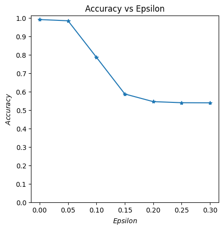
The next image summarises the models accuracy in relation to the amount of added perturbation.

Resnet8 multiclass
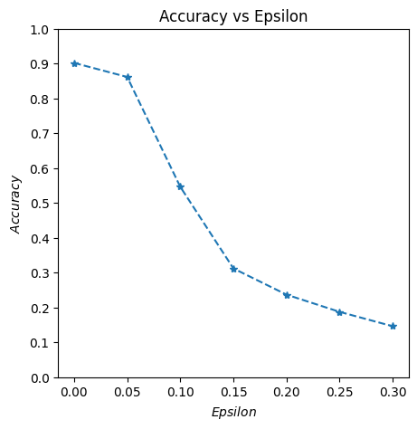
Again, some images to illustrate the effects of perturbation.
Epsilon = 0

Epsilon = 0.05

Epsilon = 0.3


Targeted
Resnet18 binary
Epsilon = 0

Epsilon = 0.3


Resnet18 multiclass
Epsilon = 0.05

Epsilon = 0.3

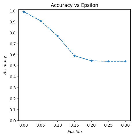
The accuracy-epsilon relationship is identical to the non-targeted case.
I’ve also tried another targeted approach. In this one I used a dynamic target class selected by picking the least likely one from the model’s initial prediction. While this seemed promising it did not deliver any better results than the previous method.
Conclusion
The targeted attack doesn't work exactly as I hoped however it seems effective as well but is not worth the extra hassle. Maybe a less covert method like adversary patches might work much better.
Code
import torch
import torch.nn as nn
import torch.nn.functional as F
import torch.optim as optim
from torchvision import datasets, transforms
import numpy as np
import matplotlib.pyplot as plt
from tqdm import tqdm
from Utilities.Util import imshow, data_transforms, image_reverse_transform
from Models.CustomModels import SimpleNet_ft, ResNet18_stock
def ResNet18_lp(num_classes: int):
    """
    Args:
        num_classes: number of output classes for the model
    Returns:
        ResNet18 model configured for linear probing (fixed feature extractor) with
        a custom head.
    """
    # pretrained model (model structure and weights)
    model = models.resnet18(weights=ResNet18_Weights.IMAGENET1K_V1)

    # replace the base model's last layer with our custom one
    # number of features being passed to the last (fully connected) layer of the base model has to be the
    # same as in base model (fc.in_features)
    # number of features we want the custom head (replaces the base model's fc) to output has to be
    # equal to num classes in our problem

    model.fc = nn.Linear(model.fc.in_features, num_classes)

    # freeze everything (weights and biases for layers cannot be updated)
    for param in model.parameters():
        param.requires_grad = False

    # unfreeze last layer (will be updated during training)
    for param in model.fc.parameters():
        param.requires_grad = True

    return model
data_dir = "./data/animals"
t = transforms.Compose(
    [
        transforms.RandomResizedCrop(224),
        transforms.RandomHorizontalFlip(),
        transforms.ToTensor(),
        transforms.Normalize([0.485, 0.456, 0.406], [0.229, 0.224, 0.225]),
    ]
)

image_datasets = datasets.ImageFolder(data_dir, transform=t)
smaller_dataset, _ = random_split(image_datasets, [0.1, 0.9])
dataloaders = torch.utils.data.DataLoader(smaller_dataset, batch_size=1, shuffle=True, num_workers=4)

dataset_sizes = len(dataloaders)*dataloaders.batch_size
class_names = image_datasets.classes
# Define what device we are using
device = torch.device("cuda" if torch.cuda.is_available() else "cpu")

model = torch.load("../Pastry_or_dogs/trained_models/best_model_params_10_classes.pth")

# Initialize the network
model = model.to(device)

# Set the model in evaluation mode. In this case this is for the Dropout layers
model.eval()
# FGSM attack code
def fgsm_attack(image, epsilon, data_grad, targeted:bool):
    # Collect the element-wise sign of the data gradient
    sign_data_grad = data_grad.sign()


    # Create the perturbed image by adjusting each pixel of the input image
    if targeted:
        perturbed_image = image - epsilon*sign_data_grad
    else:
        perturbed_image = image + epsilon*sign_data_grad

    # Adding clipping to maintain [0,1] range
    perturbed_image = torch.clamp(perturbed_image, 0, 1)
    # Return the perturbed image
    return perturbed_image


# restores the tensors to their original scale
def denorm(batch, mean, std):
    """
    Convert a batch of tensors to their original format

    Args:
        batch: batch of normalized tensors
        mean: mean used for normalization
        std: standard deviation used for normalization

    Returns:
        batch of tensors without normalization applied to them.
    """
    if isinstance(mean, list):
        mean = torch.tensor(mean).to(device)
    if isinstance(std, list):
        std = torch.tensor(std).to(device)

    return batch * std.view(1, -1, 1, 1) + mean.view(1, -1, 1, 1)
def test( model, device, loader, epsilon , mean, std, target_label = -1):

    # Accuracy counter
    correct = 0
    adv_examples = []

    # if there is a target
    if target_label != -1 and target_label != 'least_likely':
        adversary_label = torch.tensor([target_label]).to(device)
        # adversary_label = adversary_label.to(device)


    # Loop over all examples in test set
    for image, original_label in tqdm(loader):

        # Send the data and label to the device
        image, original_label = image.to(device), original_label.to(device)

        # Set requires_grad attribute of tensor. Important for Attack
        image.requires_grad = True

        # Forward pass the data through the model
        output = model(image)
        initial_prediction = output.max(1, keepdim=True)[1] # get the index of the max log-probability

        prob = F.softmax(outputs, dim=1)
        least_likely_class = prob.squeeze().cpu().numpy().argmin()


        # If the initial prediction is wrong, don't bother attacking, just move on
        if initial_prediction.item() != original_label.item():
            continue

        # targeted
        if target_label != -1 and target_label != 'least_likely':
            # Calculate the loss for targeted attack
            loss = F.nll_loss(output,adversary_label)

        # least likely class
        elif target_label == 'least_likely':
            least_likely_class = torch.tensor([least_likely_class]).to(device)
            loss = F.nll_loss(output,least_likely_class)

        # non-targeted
        else:
            # Calculate the loss for non-targeted attack
            loss = F.nll_loss(output, original_label)

        # Zero all existing gradients
        model.zero_grad()

        # Calculate gradients of model in backward pass
        loss.backward()

        # Collect ``datagrad``
        data_grad = image.grad.data

        # Restore the data to its original scale
        data_denorm = denorm(image, mean, std)
        # data_denorm = torch.tensor(data_denorm)

        # Call FGSM Attack
        perturbed_image = fgsm_attack(data_denorm, epsilon, data_grad,target_label==-1)

        # Reapply normalization
        perturbed_data_normalized = transforms.Normalize(mean, std)(perturbed_image)

        # Re-classify the perturbed image
        output = model(perturbed_data_normalized)

        # Check for success
        final_prediction = output.max(1, keepdim=True)[1] # get the index of the max log-probability
        if final_prediction.item() == original_label.item():
            correct += 1
            # Special case for saving 0 epsilon examples
            if epsilon == 0 and len(adv_examples) < 5:
                adv_ex = perturbed_image.squeeze().detach().cpu().numpy()
                og_img = data_denorm.squeeze().detach().cpu().numpy()
                adv_examples.append( (initial_prediction.item(), final_prediction.item(), adv_ex,og_img) )
        else:
            # Save some adv examples for visualization later
            if len(adv_examples) < 5:
                adv_ex = perturbed_image.squeeze().detach().cpu().numpy()
                og_img = data_denorm.squeeze().detach().cpu().numpy()
                adv_examples.append( (initial_prediction.item(), final_prediction.item(), adv_ex,og_img) )

    # Calculate final accuracy for this epsilon
    final_acc = correct/float(len(loader))
    print(f"Epsilon: {epsilon}\tTest Accuracy = {correct} / {len(loader)} = {final_acc}")

    # Return the accuracy and an adversarial example
    return final_acc, adv_examples
# amount of adjustments to the input data (amoount of pixel wise perturbation)
epsilons = [0, .05, .1, .15, .2, .25, .3]

accuracies = []
examples = []

# Run test for each epsilon
for eps in epsilons:
    acc, ex = test(model, device, dataloaders, eps, [0.485, 0.456, 0.406], [0.229, 0.224, 0.225],'least_likely')
    accuracies.append(acc)
    examples.append(ex)